%% Initialize
% set paths required for Theta Suite connection
thetaclasspath

% set workspace with the project required
theta_set_workspace('C:\Users\Andreas\ThetaSuite\workspace')

% from project "Pricing" load "bench.thetml"
thc = theta_compiler('bench.thetaml');

Then, we can set up the parameters const_l_12 to [1:40] and const_l_26 to [11:110], which is just one line of matlab meshgrid():

%% Run

% create compiler object
conf = thc.getConf();

% create grid of perameters of interest
[X,Y] = meshgrid(1:40, 11:110);

% set parameters as vectors and mark as model point using "@mp"
conf.param.const_l_12.value = {};
conf.param.const_l_12.value{1} = '@mp';
conf.param.const_l_12.value{2} = X(:);

conf.param.const_l_26.value = {};
conf.param.const_l_26.value{1} = '@mp';
conf.param.const_l_26.value{2} = Y(:);

% prepare path-wise compuation, i.e. model points in the vector
conf.generator.output_file.value = '';
conf.eval.MC.n.value = length(Y(:));
conf.VAModelpoints.PathWise.value = true;

% overwrite data if required (is also loaded from bench.thetaml)
%conf.param.data.hist.Data.value = hist_close;
%conf.param.data.hist.TimeGrid.value = yearfrac(hist_date(1), hist_date(1:end));

% set and run configuration using the theta_compiler object
thc.setConf(conf);
res = thc.run();

Render graphics in a post-process

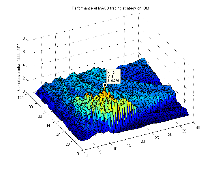
Running this script performs 4000 different performance estimations within about 60 seconds. After that, we can create nice graphics as result:

%% Plot

figure()
surf(X,Y,reshape(squeeze(res.output.Return.value(:,1,end)),100,40))
title('Performance of MACD trading strategy on IBM')
zlabel('Cumulative return 2000-2011')

figure()
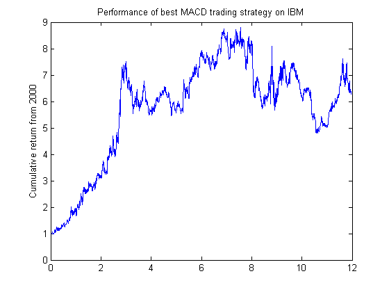
[M, I ] = max(res.output.Return.value(:,1,end));
plot(res.output.Return.time,squeeze(res.output.Return.value(I,1,:)))
title('Performance of best MACD trading strategy on IBM')
ylabel('Cumulative return from 2000')

Evaluate results

Running the plots shows the following:

and the best paths is

That means, the optimized MACD strategy was performing great during 2000 to 2003. After that time period, this strategy does not perform at all. Taking transaction costs into account, the performance is even much worse.

Conclusion

Using Matlab and Theta Suite, an efficient optimization procedure is performed. We can improve the parameters of the MACD trading strategy significantly. However, the optimized strategy only works within a short period of the historical data. This leaves you with the task to investigate other strategies: Good luck!