Besides European and American Options, another challenge in option pricing is the valuation of Barrier Options. We will see that simply applying the algorithms from the previous posts does not converge well. Especially, pricing a long-term up-and-out barrier option is hard, due to the discontinuity of the payoff. 

All posts in this series:

• Basics of a PDE solver in Matlab
• Pricing American options with a PDE solver
• Efficient pricing of barrier options

Barrier Options

In this post, we will take a look at the following barrier option:

Payoff:

• Stock price – Strike if stock price was never above barrier level .
• otherwise.

That means, the value for is zero. First, we try to introduce this in an explicit constraint. We use the  condition in the PDE solver (How Can I Price an Option with a PDE Method in Matlab?) and change the solver loop:

for tau=1:time_steps
   V = M\ V;
   V(S>=H)=0;
end

Analyzing the convergence of the solver with explicit constraint

Now, we take a look at a numerical example. In the following, we price an up-and-out Barrier option with , , , ,  and . Using different levels of “refine” with the PDE solver and the explicit constraint, we obtain the following values:

 refine        V_res   Difference       Factor
      1   0.05571209            0            0
      2   0.07059614   0.01488404            0
      3   0.07385265   0.00325651   4.57054309
      4   0.07434690   0.00049424   6.58891052
      5   0.07402224  -0.00032465  -1.52237808
      6   0.07343880  -0.00058344   0.55643959
      7   0.07281298  -0.00062581   0.93229160

This table presents the option values for different levels of “refine”. The column “Difference” presents the difference between two refine levels and the column “Factor” presents the factor between the “Difference” of two levels of refine.

We can see that absolute values of factor changes between 0.5 and 6.5, i.e. the error does not decrease smoothly for higher levels.

Improving convergence using an implicit barrier constraint

The idea for improving the convergence is an implicit introduction of the constraint, similar to the penalty method for American options. I.e. we introduce an additional equation into

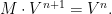
We want to force numerically . This can be done e.g. by the introduction of a penalty in the equation.

Then, the solver loop is:

    for tau=1:time_steps
        P(S>=H)=100000;
        V = (M + diag(P))\V
    end

Analyzing the convergence of the solver with implicit constraint

Analyzing the convergence of the solver, we increase “refine” from 1 to 7 and then take a close look at the results.

 refine        V_res   Difference       Factor
      1   0.05269513            0            0
      2   0.06639892   0.01370379            0
      3   0.06940017   0.00300124   4.56602960
      4   0.07011419   0.00071402   4.20327399
      5   0.07028354   0.00016934   4.21631141
      6   0.07032179   0.00003824   4.42771568
      7   0.07032934   0.00000754   5.06592917

In this table, the factor between different refine levels is between 4 and 5. This is a good result: It shows that doubling the nodes in the mesh for and doubling the number of time steps reduces the error to 1/4. This is called quadratic convergence. By the way, the real option value can be obtained from an analytic solution of the Barrier Option is .

Implementation

Here is the Matlab PDE solver for Barrier options:

% init S with a structured mesh
clear;
refine = 7;
explicit = false; % change to true for explicit handling of constraint

sigma = 0.4;
r = 0.05;
K = 100;
T = 2;
H = 120;
LargePenalty = 100000;

S = [0 60:20:160 200 1000];
for iterRefine=1:refine
    if refine >1
        Sn(1:2:length(S)*2) = S;
        Sn(2:2:length(S)*2-1) = (S(2:length(S)) -S(1:length(S)-1))/2 + S(1:length(S)-1);
        S = Sn;
    end

    time_steps = round(256 *2^(iterRefine-1)* T);
    dtau = T/time_steps;

    V = max(S'-K,0); % V(t=T) = payoff at maturity
    V(S>=H) = 0;     % no value above barrier

    Sm = S(1:length(S)-2);
    Si = S(2:length(S)-1);
    Sp = S(3:length(S));

    m_i = 1 + (sigma^2*Si.^2*dtau).*(1./( (Sp-Sm).*(Sp-Si) ) +1./( (Sp-Sm).*(Si-Sm) ) ) + r*dtau;
    m_i = [1+r*dtau m_i 1]; % boundary
    m_iplus =-(sigma^2*Si.^2*dtau)./((Sp-Sm).*(Sp-Si)) - Si.*r*dtau./(Sp-Sm);
    m_iminus = -(sigma^2*Si.^2*dtau)./((Sp-Sm).*(Si-Sm)) + Si.*r*dtau./(Sp-Sm);

    M = spdiags([ [m_iminus 0 0]; m_i; [0 0 m_iplus]]', -1:1, length(m_i), length(m_i));
    P = zeros(length(S),1);

    for tau=1:time_steps
        if explicit
           V = M\ V;
           V(S>=H)=0;
        else
           P(S>=H)=LargePenalty;
           % equivalent but more efficient than V = (M + diag(P))\V
           V = (M + spdiags(P,0,length(V),length(V))) \ V;
        end
    end
    % save value at S=100 for convergence study
    V_res(iterRefine,1) = V(S==100);
end

%%
V_diff   = V_res(2:end)-V_res(1:end-1);
V_factor = V_diff(1:end-1)./V_diff(2:end);

V_diff   = [0; V_diff];
V_factor = [0; 0; V_factor];

indexRefine = [1:refine]';
disp([indexRefine V_res V_diff V_factor])

Conclusion

Using a penalty method, the PDE solver can efficiently handle barrier options. The numerical example shows that an up-and-out barrier option can be priced with quadratic convergence.